Random Forest Classification

The classification step consists in one or many numerical processes to finally allocate every pixel or object to one of the classes of the land cover typology. The vast diversity of classification algorithms can be split into two main types:

• the supervised type, which uses a training data set to calibrate the algorithm a priori;

• and the unsupervised type, which produces clusters of pixels to be labelled a posteriori as land cover class in light of in situ or ancillary information.

Random Forest (RF), an improved implementation of Decision Trees (DT), is an ensemble-learning algorithm that combines multiple classifications of the same data to produce higher classification accuracies than other forms of DT. RF works by fitting many DT-based classifications to a data set, and then uses a rule-based approach to combine the predictions from all the trees. During this process, individual trees are grown from differing subsets of training data using a process called “bagging”. Bagging involves the random subsampling (with replacement) of the original data for growing each tree. Generally, for each tree grown, two thirds of the training data are used to grow the tree, while the remaining one third are left unused (out-of-bag, or OOB) for later error assessment. A classification is then fit to each bootstrap sample; however, at each node (split), only a small number of randomly selected predictor variables are used in the binary partitioning. The splitting process continues until further subdivision no longer reduces the Gini index. Each tree contributes to the assignment of the most frequent class to the input data with a single vote. The predicted class of an observation is calculated by the majority vote for that observation, with ties split randomly.

The random forest combines hundreds or thousands of decision trees, trains each one on a slightly different set of the observations, splitting nodes in each tree considering a limited number of the features. The final predictions of the random forest are made by averaging the predictions of each individual tree.

Watch this video if Decision Trees are not clear for you !

Watch this video if Random Forest are not clear for you !

In this chapter we will see how to use the Random Forest implementation provided by the scikit-learn library. Scikit-learn is an amazing machine learning library that provides easy and consistent interfaces to many of the most popular machine learning algorithms. It is built on top of the pre-existing scientific Python libraries, including NumPy, SciPy, and matplotlib, which makes it very easy to incorporate into your workflow. The number of available methods for accomplishing any task contained within the library is its real strength.

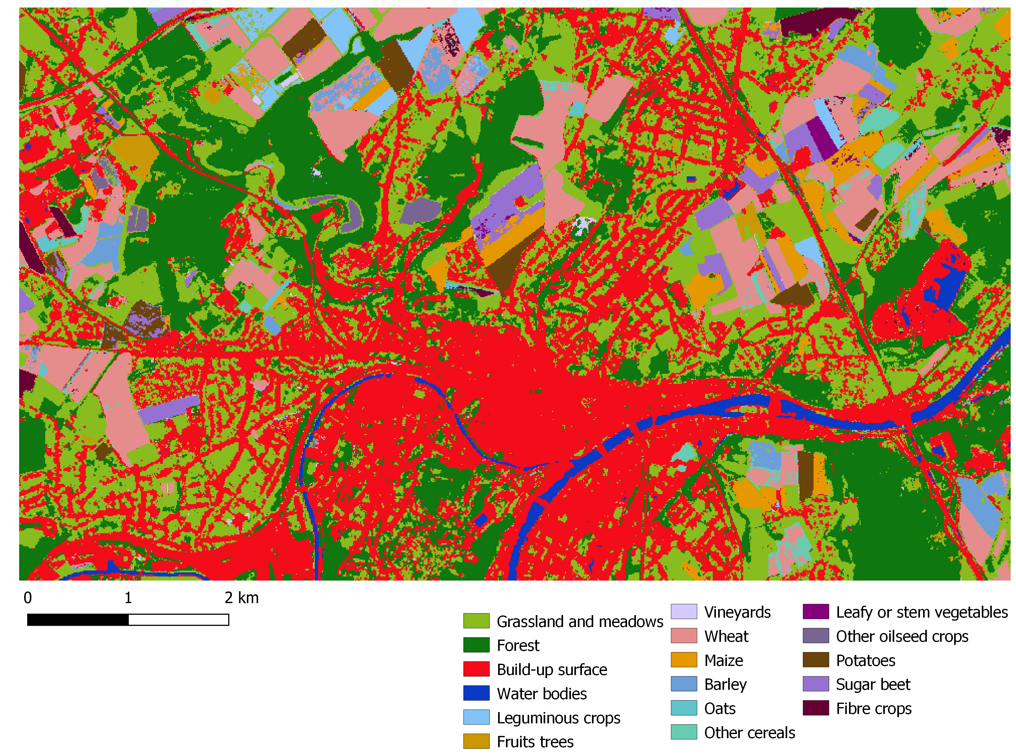
Namur, 2020 (NDVI & monthly composites S1 backscattering VV)

---

Handbook on remote sensing for agricultural statistics

Chris Holden’s tutorial

An Implementation and Explanation of the Random Forest in Python

import glob, os, time, math
import numpy as np
import pandas as pd
import geopandas as gpd
import rasterio
import rasterio.plot
from rasterio import features

import sklearn
from sklearn.ensemble import RandomForestClassifier

from pathlib import Path
from IPython.display import display

print('All libraries successfully imported!')
print(f'Scikit-learn : {sklearn.__version__}')

All libraries successfully imported!
Scikit-learn : 1.2.0

Set directory

computer_path = 'X:/'
grp_nb        = '99'

data_path = f'{computer_path}data/'                        # Directory with data shared by the assistant
work_path = f'{computer_path}STUDENTS/GROUP_{grp_nb}/'  # Directory for all work files

# Input directories
in_situ_path = f'{work_path}C_IN_SITU_CAL_VAL/'
s2_path      = f'{work_path}3_L2A_MASKED/'
ndvi_path    = f'{work_path}NDVI/'
s1_path      = f'{data_path}S1_GRD/'
lut_path     = f'{data_path}LUT/'

# Output directory
classif_path = f'{work_path}CLASSIF/'

Path(classif_path).mkdir(parents=True, exist_ok=True)

print(f'Classification path is set to : {classif_path}')

Classification path is set to : /export/miro/ndeffense/LBRAT2104/STUDENTS/GROUP_99/TP/CLASSIF/

Set parameters

site = 'NAMUR'
year = '2020'

no_data = -999

ws = 3 # Must be a odd number 3x3, 5x5, 7x7, ... (filtering post classification)

# Field used for classification
field_classif_code = 'grp_1_nb'
field_classif_name = 'grp_1'

# Field used for reclassification
field_reclassif_code = 'grp_A_nb'
field_reclassif_name = 'grp_A'

# Group of features used in classification
feat_nb = 2

if feat_nb == 1:
    feat_name = ['NDVI']
elif feat_nb == 2:
    feat_name = ['NDVI','S1_monthly_mean']

Set filenames

Input files

in_situ_cal_shp = f'{in_situ_path}{site}_{year}_IN_SITU_ROI_CAL.shp'

s4s_lut_xlsx = f'{lut_path}crop_dictionary.xlsx'

Output files

in_situ_cal_tif = f'{in_situ_path}{site}_{year}_IN_SITU_ROI_CAL.tif'

classif_tif          = f'{classif_path}{site}_{year}_classif_RF_feat_{feat_nb}_{field_classif_name}.tif'
reclassif_tif        = f'{classif_path}{site}_{year}_classif_RF_feat_{feat_nb}_{field_classif_name}_reclassify_{field_reclassif_name}.tif'
reclassif_filter_tif = f'{classif_path}{site}_{year}_classif_RF_feat_{feat_nb}_{field_classif_name}_reclassify_{field_reclassif_name}_filter_ws_{ws}x{ws}.tif'

1. Prepare classification features associated to in situ data

1.1 Rasterize in situ data calibration shapefile

# Open the calibration polygons with GeoPandas
in_situ_gdf = gpd.read_file(in_situ_cal_shp)

# Open the raster file you want to use as a template for rasterize
img_temp_tif = glob.glob(f'{s2_path}*.tif')[0]

print(f'Raster template file : {img_temp_tif}')

src = rasterio.open(img_temp_tif, "r")

# Update metadata

out_meta = src.meta
out_meta.update(nodata=no_data)

crs_shp = str(in_situ_gdf.crs).split(":",1)[1]
crs_tif = str(src.crs).split(":",1)[1]

print(f'The CRS of in situ data is    : {crs_shp}')
print(f'The CRS of raster template is : {crs_tif}')

if crs_shp == crs_tif:
    print("CRS are the same")

    print(f'Rasterize starts : {in_situ_cal_shp}')

    # Burn the features into the raster and write it out

    dst = rasterio.open(in_situ_cal_tif, 'w+', **out_meta)
    dst_arr = dst.read(1)

    # This is where we create a generator of geom, value pairs to use in rasterizing

    geom_col = in_situ_gdf.geometry
    code_col = in_situ_gdf[field_classif_code].astype(int)

    shapes = ((geom,value) for geom, value in zip(geom_col, code_col))

    in_situ_arr = features.rasterize(shapes=shapes,
                                     fill=no_data,
                                     out=dst_arr,
                                     transform=dst.transform)

    dst.write_band(1, in_situ_arr)

    print(f'Rasterize is done : {in_situ_cal_tif}')

    # Close rasterio objects
    src.close()
    dst.close()

else:
    print('CRS are different --> repoject in-situ data shapefile with "to_crs"')

Raster template file : /export/miro/ndeffense/LBRAT2104/STUDENTS/GROUP_99/TP/3_L2A_MASKED/T31UFS_20200116T105309_B02_10m_ROI_SCL.tif
The CRS of in situ data is    : 32631
The CRS of raster template is : 32631
CRS are the same
Rasterize starts : /export/miro/ndeffense/LBRAT2104/STUDENTS/GROUP_99/TP/C_IN_SITU_CAL_VAL/NAMUR_2020_IN_SITU_ROI_CAL.shp
Rasterize is done : /export/miro/ndeffense/LBRAT2104/STUDENTS/GROUP_99/TP/C_IN_SITU_CAL_VAL/NAMUR_2020_IN_SITU_ROI_CAL.tif

1.2 List all the classification features

Create an empty list to append all feature rasters one by one

list_src_arr = []

1 NDVI image per month

if 'NDVI' in feat_name:

    list_im = sorted(glob.glob(f'{ndvi_path}*.tif'))

    for im_file in list_im:

        src = rasterio.open(im_file, "r")
        im = src.read(1)
        list_src_arr.append(im)
        src.close()

    print(f'Shape of features : {im.shape}')
    print(f'Number of features : {len(list_src_arr)}')

else:
    print("No NDVI in the set of features")

Shape of features : (570, 986)
Number of features : 12

S1 monthly mean composite (obtained with Google Earth Engine)

if 'S1_monthly_mean' in feat_name:

    s1_montlhy_mean_tif = f'{s1_path}monthly_mean_{site}_{year}.tif'

    src = rasterio.open(s1_montlhy_mean_tif, "r")
    im = src.read()
    src.close()

    for i in range(len(im)):
        band = im[i]
        list_src_arr.append(band)

    print(f'Shape of features : {band.shape}')
    print(f'Number of features : {len(list_src_arr)}')

else:
    print("No S1 monthly mean in the set of features")

Shape of features : (570, 986)
Number of features : 24

Merge all the 2D matrices from the list into one 3D matrix

feat_arr = np.dstack(list_src_arr).astype(np.float32)

print(feat_arr.shape)
print(f'There are {feat_arr.shape[2]} features')
print(f'The features type is : {feat_arr.dtype}')

#feat_arr_1 = np.stack(list_src_arr, axis=0)
#print(feat_arr_1.shape)

(570, 986, 24)
There are 24 features
The features type is : float32

1.3 Pairing in situ data (Y) with EO classification features (X)

Now that we have the image we want to classify (our X feature inputs), and the ROI with the land cover labels (our Y labeled data), we need to pair them up in NumPy arrays so we may feed them to Random Forest.

# Open in-situ used for calibration

src = rasterio.open(in_situ_cal_tif, "r")
cal_arr = src.read(1)
src.close()

# Find how many labeled entries we have -- i.e. how many training data samples?
n_samples = (cal_arr != no_data).sum()

print(f'We have {n_samples} samples (= calibration pixels)')

We have 34909 samples (= calibration pixels)

What are our classification labels?

labels = np.unique(cal_arr[cal_arr != no_data])

print(f'The training data include {labels.size} classes: {labels}')

The training data include 19 classes: [   3   21   22   69   81   84  121 1111 1121 1152 1171 1192 1435 1511
 1771 1811 1911 1923 9212]

We need :

• “X” 2D matrix containing classification features

• “y” 1D matrix containing our labels

These will have n_samples rows.

X = feat_arr[cal_arr != no_data, :]
y = cal_arr[cal_arr != no_data]

# Replace NaN in classification features by the no_data value
X = np.nan_to_num(X, nan=no_data)

print(f'Our X matrix is sized: {X.shape}')
print(f'Our y array is sized: {y.shape}')

Our X matrix is sized: (34909, 24)
Our y array is sized: (34909,)

2. Train the Random Forest

Now that we have our X 2D-matrix of feature inputs and our y 1D-matrix containing the labels, we can train our model.

Visit this web page to find the usage of RandomForestClassifier from scikit-learn.

start_training = time.time()

# Initialize our model
rf = RandomForestClassifier(n_estimators=100, # The number of trees in the forest.
                            bootstrap=True,   # Whether bootstrap samples are used when building trees. If False, the whole dataset is used to build each tree.
                            oob_score=True)   # Whether to use out-of-bag samples to estimate the generalization score. Only available if bootstrap=True.

# Fit our model to training data
rf = rf.fit(X, y)

end_training = time.time()

# Get time elapsed during the Random Forest training
hours, rem = divmod(end_training-start_training, 3600)
minutes, seconds = divmod(rem, 60)
print("Random Forest training : {:0>2}:{:0>2}:{:05.2f}".format(int(hours),int(minutes),seconds))

Random Forest training : 00:00:13.95

With our Random Forest model fit, we can check out the “Out-of-Bag” (OOB) prediction score.

Score of the training dataset obtained using an out-of-bag estimate. This attribute exists only when oob_score is True.

print(f'Our OOB prediction of accuracy is: {round(rf.oob_score_ * 100,2)}%')

Our OOB prediction of accuracy is: 99.49%

To help us get an idea of which features bands were important, we can look at the feature importance scores.

The impurity-based feature importances. The higher, the more important the feature. The importance of a feature is computed as the (normalized) total reduction of the criterion brought by that feature. It is also known as the Gini importance.

feat_band_list = []
gini_list      = []

for band_nb, imp in enumerate(rf.feature_importances_, start=1):

    feat_band_list.append(band_nb)
    gini_list.append(imp)

gini_dict = {'feat_band':feat_band_list,'Gini':gini_list}

gini_df = pd.DataFrame(gini_dict).round(4)

feat_name_df = pd.read_excel(f'{data_path}feature_name.xlsx')

gini_df = feat_name_df.merge(gini_df, on='feat_band').sort_values(by='Gini', ascending=False)

gini_df

	feat_band	feat_name	Gini
6	7	NDVI July	0.0994
7	8	NDVI August	0.0885
4	5	NDVI May	0.0871
8	9	NDVI September	0.0784
3	4	NDVI April	0.0722
2	3	NDVI March	0.0702
0	1	NDVI January	0.0555
17	18	S1 mean composite - June	0.0479
9	10	NDVI October	0.0476
18	19	S1 mean composite - July	0.0447
10	11	NDVI November	0.0427
11	12	NDVI December	0.0320
19	20	S1 mean composite - August	0.0318
16	17	S1 mean composite - May	0.0305
15	16	S1 mean composite - April	0.0302
5	6	NDVI June	0.0285
1	2	NDVI February	0.0213
20	21	S1 mean composite - September	0.0194
12	13	S1 mean composite - January	0.0173
13	14	S1 mean composite - February	0.0128
23	24	S1 mean composite - December	0.0118
14	15	S1 mean composite - March	0.0113
21	22	S1 mean composite - October	0.0101
22	23	S1 mean composite - November	0.0088

Let’s look at a crosstabulation to see the class confusion

# Setup a dataframe
df = pd.DataFrame()

df['truth'] = y
df['predict'] = rf.predict(X)

# Cross-tabulate predictions

cross_tab = pd.crosstab(df['truth'], df['predict'], margins=True)
display(cross_tab)

predict	3	21	22	69	81	84	121	1111	1121	1152	1171	1192	1435	1511	1771	1811	1911	1923	9212	All
truth
3	5971	0	0	0	0	0	0	0	0	0	0	0	0	0	0	0	0	0	0	5971
21	0	1551	0	0	0	0	0	0	0	0	0	0	0	0	0	0	0	0	0	1551
22	0	0	124	0	0	0	0	0	0	0	0	0	0	0	0	0	0	0	0	124
69	0	0	0	2296	0	0	0	0	0	0	0	0	0	0	0	0	0	0	0	2296
81	0	0	0	0	1338	0	0	0	0	0	0	0	0	0	0	0	0	0	0	1338
84	0	0	0	0	0	183	0	0	0	0	0	0	0	0	0	0	0	0	0	183
121	0	0	0	0	0	0	566	0	0	0	0	0	0	0	0	0	0	0	0	566
1111	0	0	0	0	0	0	0	7403	0	0	0	0	0	0	0	0	0	0	0	7403
1121	0	0	0	0	0	0	0	0	2132	0	0	0	0	0	0	0	0	0	0	2132
1152	0	0	0	0	0	0	0	0	0	1663	0	0	0	0	0	0	0	0	0	1663
1171	0	0	0	0	0	0	0	0	0	0	534	0	0	0	0	0	0	0	0	534
1192	0	0	0	0	0	0	0	0	0	0	0	1477	0	0	0	0	0	0	0	1477
1435	0	0	0	0	0	0	0	0	0	0	0	0	1176	0	0	0	0	0	0	1176
1511	0	0	0	0	0	0	0	0	0	0	0	0	0	1577	0	0	0	0	0	1577
1771	0	0	0	0	0	0	0	0	0	0	0	0	0	0	2454	0	0	0	0	2454
1811	0	0	0	0	0	0	0	0	0	0	0	0	0	0	0	1850	0	0	0	1850
1911	0	0	0	0	0	0	0	0	0	0	0	0	0	0	0	0	403	0	0	403
1923	0	0	0	0	0	0	0	0	0	0	0	0	0	0	0	0	0	2059	0	2059
9212	0	0	0	0	0	0	0	0	0	0	0	0	0	0	0	0	0	0	152	152
All	5971	1551	124	2296	1338	183	566	7403	2132	1663	534	1477	1176	1577	2454	1850	403	2059	152	34909

Unbelievable? I highly doubt the real confusion matrix will be 100% accuracy. What is likely going on is that we used a large number of trees within a machine learning algorithm to best figure out the pattern in our training data. Given enough information and effort, this algorithm precisely learned what we gave it. Asking to validate a machine learning algorithm on the training data is a useless exercise that will overinflate the accuracy.

Instead, we could have done a crossvalidation approach where we train on a subset the dataset, and then predict and assess the accuracy using the sections we didn’t train it on.

3. Predict the rest of the image

With our Random Forest classifier fit, we can now proceed by trying to classify the entire image.

# Take our full image and reshape into long 2d array (nrow * ncol, nband) for classification

img = feat_arr

img = np.nan_to_num(img, nan=no_data)

new_shape = (img.shape[0] * img.shape[1], img.shape[2])

img_as_array = img[:, :, :].reshape(new_shape)

print(img_as_array)

print(f'Reshaped from {img.shape} to {img_as_array.shape}')

start_classification = time.time()

# Now predict for each pixel
class_prediction = rf.predict(img_as_array)

# Reshape our classification map
class_prediction = class_prediction.reshape(img[:, :, 0].shape)

end_classification = time.time()

hours, rem = divmod(end_classification-start_classification, 3600)
minutes, seconds = divmod(rem, 60)
print("Random Forest training : {:0>2}:{:0>2}:{:05.2f}".format(int(hours),int(minutes),seconds))

print(class_prediction)

[[ 6.60263658e-01  4.29129243e-01  6.68883979e-01 ... -1.23333731e+01
  -1.23078318e+01 -1.07777815e+01]
 [ 5.07605612e-01  4.32377875e-01  5.90189874e-01 ... -9.39306545e+00
  -1.21026096e+01 -1.09584541e+01]
 [ 4.00820792e-01  3.75474095e-01  4.71971065e-01 ... -8.66642475e+00
  -1.05296297e+01 -1.01824131e+01]
 ...
 [-9.99000000e+02 -9.99000000e+02 -9.99000000e+02 ... -7.79056311e+00
  -8.99753094e+00 -9.10786438e+00]
 [-9.99000000e+02 -9.99000000e+02 -9.99000000e+02 ... -8.75600719e+00
  -8.76734066e+00 -9.15415192e+00]
 [-9.99000000e+02 -9.99000000e+02 -9.99000000e+02 ... -1.01634216e+01
  -9.73724937e+00 -9.64400387e+00]]
Reshaped from (570, 986, 24) to (562020, 24)
Random Forest training : 00:00:09.11
[[   3   21   81 ...    3    3    3]
 [   3   21   21 ...    3    3    3]
 [   3    3   21 ...    3    3 1121]
 ...
 [  69   69   69 ... 1111 1111 1111]
 [  69   69   69 ... 1111 1111 1111]
 [  81   81   81 ...   81 9212   81]]

4. Reclassify classification

4.1 Open LUT and sort values

lut_df = pd.read_excel(s4s_lut_xlsx)

lut_df = lut_df.sort_values(by=field_classif_code, ascending=True)

display(lut_df[[field_classif_code, field_classif_name, field_reclassif_code, field_reclassif_name]].head())

	grp_1_nb	grp_1	grp_A_nb	grp_A
0	0	Remove	0	Remove
71	0	Remove	0	Remove
75	0	Remove	0	Remove
82	0	Remove	0	Remove
86	0	Remove	0	Remove

4.2 Reclassify prediction

reclass_prediction = np.copy(class_prediction)

for i, row in lut_df.iterrows():

    old_class = row[field_classif_code]
    new_class = row[field_reclassif_code]

    #print(f'{old_class} --> {new_class}')

    #array[np.where(array == old_class)] = new_class

    reclass_prediction[reclass_prediction == old_class] = new_class

print(f'Classification : \n {class_prediction}')
print(f'Re-classification : \n {reclass_prediction}')

Classification :
 [[   3   21   81 ...    3    3    3]
 [   3   21   21 ...    3    3    3]
 [   3    3   21 ...    3    3 1121]
 ...
 [  69   69   69 ... 1111 1111 1111]
 [  69   69   69 ... 1111 1111 1111]
 [  81   81   81 ...   81 9212   81]]
Re-classification :
 [[  3  21   8 ...   3   3   3]
 [  3  21  21 ...   3   3   3]
 [  3   3  21 ...   3   3 112]
 ...
 [  6   6   6 ... 111 111 111]
 [  6   6   6 ... 111 111 111]
 [  8   8   8 ...   8   9   8]]

5. Filter classification with moving window

sizey = reclass_prediction.shape[0]
sizex = reclass_prediction.shape[1]

rad_wind = math.floor(ws/2)

X = np.pad(reclass_prediction, ((rad_wind,rad_wind),(rad_wind,rad_wind)), 'edge')

majority = np.empty((sizey,sizex), dtype='int16')

for i in range(sizey):
    for j in range(sizex):
        window = X[i:i+ws , j:j+ws]
        window = window.flatten()
        counts = np.bincount(window)
        maj = np.argmax(counts)
        majority[i,j]= maj


majority = majority.reshape((1,sizey,sizex))

print(f'Re-classification : \n {reclass_prediction}')
print(f'Re-classification with filter : \n {majority}')

Re-classification :
 [[  3  21   8 ...   3   3   3]
 [  3  21  21 ...   3   3   3]
 [  3   3  21 ...   3   3 112]
 ...
 [  6   6   6 ... 111 111 111]
 [  6   6   6 ... 111 111 111]
 [  8   8   8 ...   8   9   8]]
Re-classification with filter :
 [[[  3  21   8 ...   3   3   3]
  [  3   3  21 ...   3   3   3]
  [  3   3   3 ...   3   3 112]
  ...
  [  6   6   6 ... 111 111 111]
  [  6   6   6 ... 111 111 111]
  [  8   8   8 ...   8   8   8]]]

6. Write classification products into GeoTIFF files

Open template image to get metadata

with rasterio.open(img_temp_tif) as src:
    profile = src.profile

profile

{'driver': 'GTiff', 'dtype': 'int16', 'nodata': -10000.0, 'width': 986, 'height': 570, 'count': 1, 'crs': CRS.from_epsg(32631), 'transform': Affine(10.0, 0.0, 627260.0,
       0.0, -10.0, 5596180.0), 'blockysize': 4, 'tiled': False, 'compress': 'lzw', 'interleave': 'band'}

Write classification

with rasterio.open(classif_tif, "w", **profile) as dst:
    dst.write(class_prediction, 1)

Write re-classification

with rasterio.open(reclassif_tif, "w", **profile) as dst:
    dst.write(reclass_prediction, 1)

Write re-classification with moving window filtering

with rasterio.open(reclassif_filter_tif, "w", **profile) as dst:
    dst.write(majority)